Understanding Weighting Curves and Human Perception

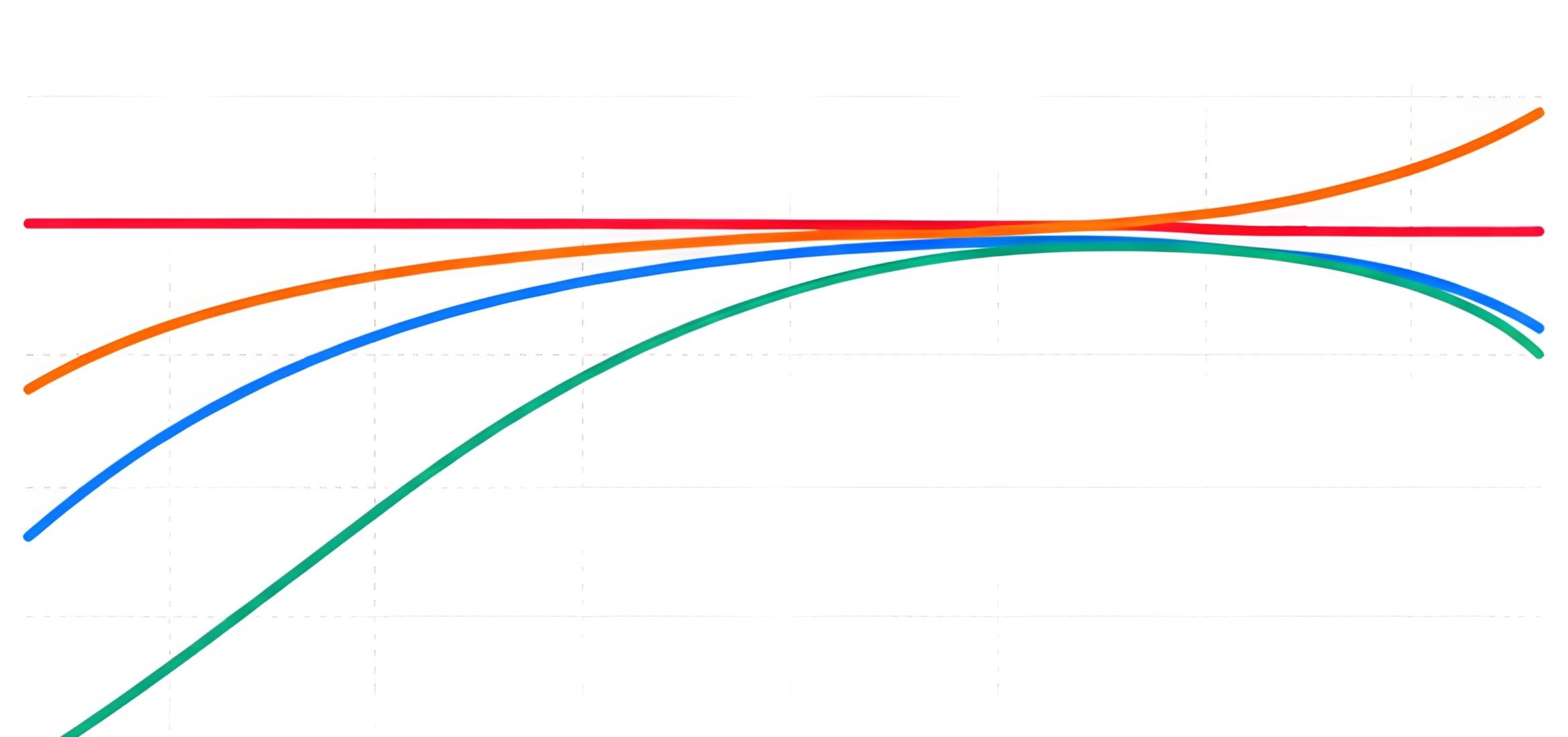
Weighting curves help audio meters measure sound in a way that better matches human hearing. Instead of treating every frequency equally, they emphasize or reduce different frequency ranges before calculating the final level.

That matters because our ears are not flat measurement devices. We hear midrange frequencies very efficiently, while deep bass and extreme treble usually need more energy to appear equally loud. As a result, two sounds with the same physical level can feel completely different.

For music producers, mastering engineers, DJs, podcasters, and broadcasters, understanding weighting curves makes meter readings far more useful. It also helps explain the difference between measurements such as dB(A), dB(C), dB(Z), LUFS, and LKFS.

Table of Contents

1. What Are Weighting Curves?
2. The Main Sound Weighting Curves
3. Loudness Weighting Curves and K-Weighting
4. Using Weighting Curves in Music Production
5. Weighting Curves for DJs and Live Sound
6. Weighting Curves for Podcasts
7. Weighting Curves in Broadcast
8. Common Weighting Curve Mistakes
9. A Practical Measurement Workflow
10. Final Thoughts on Weighting Curves

What Are Weighting Curves?

Weighting curves are frequency filters placed inside a measurement system. The meter applies the selected curve to the incoming signal before calculating its final reading.

Imagine measuring a bass-heavy club track with a completely flat meter. The sub-bass may contain a huge amount of physical energy. However, your ears are less sensitive to that energy than they are to a vocal around 2 or 3 kHz.

A weighted measurement compensates for this difference. It does not change the sound coming from the speakers. Instead, it changes how the meter interprets that sound.

A meter is useful only when you understand what it is designed to ignore.

Different weighting curves answer different questions. One curve may estimate hearing exposure. Another may measure powerful low-frequency peaks. A third may calculate the perceived loudness of an entire song or broadcast programme.

Why Human Hearing Needs a Frequency-Dependent Measurement

Human hearing changes dramatically across the frequency spectrum. We are especially sensitive around the upper midrange, where speech intelligibility and many important warning sounds are located.

We are much less sensitive to very low frequencies. For example, a 50 Hz tone normally needs considerably more sound pressure than a 1 kHz tone before both appear equally loud.

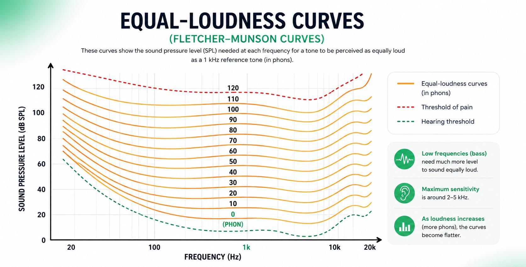
These relationships are represented by equal-loudness contours. The current scientific reference is ISO 226:2023, which defines combinations of frequencies and sound pressure levels that listeners perceive as equally loud under controlled conditions.

Equal-loudness contours also change with level. At quiet playback levels, bass and treble appear relatively weak. As playback becomes louder, the perceived response of the ear becomes flatter.

This is one reason a mix can sound balanced at high volume but thin when played quietly. It is also why checking a mix at several monitoring levels remains useful, even when you have accurate meters.

For a more visual introduction to the relationship between equal-loudness contours and acoustic measurements, this overview from Atelier Crescendo provides useful background.

Weighting Curves Are Not Normal EQ

A weighting curve may look like an EQ curve, but its purpose is different. Normal EQ changes the audio that listeners hear. Measurement weighting changes only the signal entering the meter.

For example, selecting A-weighting on a sound level meter does not remove bass from your studio monitors. It tells the meter to count low-frequency energy less heavily when producing its final number. This distinction is essential:

• EQ changes the programme material.
• Weighting changes the measurement.
• Loudness normalization changes playback gain.

Confusing these three processes can lead to poor decisions. A low A-weighted reading does not automatically mean that your track needs more midrange. Likewise, a high LUFS reading does not reveal which frequency range is causing the problem.

The Main Sound Weighting Curves

The most common acoustic weighting curves are A, C, and Z. Each one treats the frequency spectrum differently and is suited to a different type of measurement.

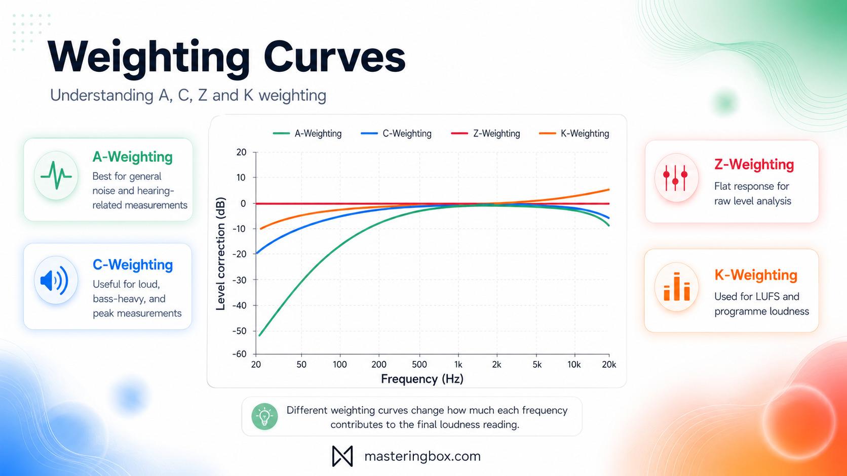
A-weighting is widely used for environmental noise and hearing exposure. C-weighting retains much more low-frequency information. Z-weighting is effectively flat.

These curves form part of standardized sound-level measurement systems such as those described in IEC 61672-1.

A-Weighting

A-weighting is probably the best-known acoustic weighting curve. Measurements made with it are normally written as dB(A), dBA, or LAeq, depending on the meter and the type of averaging being used.

The curve strongly reduces deep bass. It also reduces the highest audible frequencies, while leaving the midrange relatively prominent. At 1 kHz, its adjustment is defined as 0 dB.

Historically, A-weighting was designed as a simplified approximation of human sensitivity at moderate sound levels. However, it should not be treated as a perfect simulation of hearing.

Real hearing changes with level, duration, signal type, age, and the individual listener. A-weighting is fixed. It applies the same filter whether you are measuring conversation, machinery, or a kick drum.

Where A-Weighting Is Useful

A-weighting is most useful when the goal is to estimate general noise exposure or compare measured levels against regulations. Common applications include:

• Workplace noise exposure
• Venue noise restrictions
• Environmental noise reports
• Equipment noise specifications
• Hearing-conservation measurements
• Long-term average SPL monitoring

The NIOSH occupational noise guidance, for example, defines a recommended exposure limit of 85 dB(A) averaged across an eight-hour working day. It also halves the recommended exposure duration for each 3 dB increase.

That does not mean 85 dB(A) is automatically safe in every situation. Exposure duration matters. So do repeated sessions, recovery time, and individual susceptibility.

For producers and DJs, the practical lesson is simple: monitoring level and listening time must be considered together.

Where A-Weighting Can Mislead You

A-weighting can underrepresent bass-heavy sound. A club system may produce powerful sub-bass while the A-weighted reading appears less dramatic than expected. Therefore, do not use dB(A) alone to evaluate:

• Subwoofer headroom
• Low-frequency system stress
• Bass balance in a mix
• Short, high-energy peaks
• The tonal balance of a master

In music production, A-weighting is better used for monitoring exposure than for deciding whether your bass guitar is loud enough.

C-Weighting

C-weighting produces a much flatter measurement than A-weighting. It still reduces frequencies at the extreme ends of the spectrum, but it keeps far more bass energy in the final result. Measurements are normally written as dB(C) or dBC.

C-weighting is useful for loud, bass-heavy environments because low frequencies contribute much more strongly to its reading. A large subwoofer peak that barely changes an A-weighted average may produce a clear increase on a C-weighted meter.

Where C-Weighting Is Useful

C-weighting is commonly used when low-frequency content and strong peaks need to remain visible. Typical applications include:

• Concert and nightclub monitoring
• Subwoofer evaluation
• Peak sound-pressure measurements
• Cinema and studio calibration
• Bass-heavy machinery or environmental noise
• Comparing dB(A) and dB(C) readings

The difference between the A-weighted and C-weighted readings can be informative. A large gap often indicates substantial low-frequency energy.

However, it is not a detailed spectral analysis. Two very different frequency balances may still produce a similar difference between dB(A) and dB(C).

For monitor calibration, engineers commonly use band-limited pink noise, one speaker at a time, with the meter set to C-weighting and slow response. The exact target level depends on room size, listening distance, and the production environment.

Z-Weighting

Z-weighting means zero frequency weighting. Within the specified measurement range, the meter applies no perceptual compensation. Measurements are usually written as dB(Z) or dBZ.

Z-weighting is useful when you want the meter to report the acoustic signal without deliberately reducing bass or treble. It is the closest of these three curves to a flat measurement. Common uses include:

• Measuring raw sound pressure
• Technical equipment tests
• Frequency-response analysis
• Capturing low-frequency energy
• Comparing weighted and unweighted readings
• Investigating unexpected peaks

Z-weighting still depends on the microphone, preamp, meter bandwidth, calibration, and acoustic environment. “Unweighted” does not mean “perfectly accurate under every condition.”

Other Weighting Curves

Several other curves exist, although they are less relevant to everyday music production.

• B-weighting was intended for intermediate listening levels. It is now largely obsolete.
• D-weighting was developed for aircraft noise. Its shape gives additional importance to frequencies associated with perceived jet-engine noise.
• G-weighting is used for infrasound, including frequencies below the normal audible range.

These curves are valuable in their intended fields. However, most producers will work mainly with A, C, Z, and K-weighting.

Loudness Weighting Curves and K-Weighting

Acoustic SPL measurements and digital loudness measurements are related, but they are not interchangeable. A-weighting and C-weighting normally operate on sound captured by a calibrated microphone. K-weighting usually operates directly on a digital audio signal.

K-weighting is used by modern LUFS and LKFS meters. It forms part of the loudness algorithm defined by ITU-R BS.1770-5.

This is the system behind many broadcast, podcast, video, and music loudness workflows.

How K-Weighting Works

K-weighting applies two main filtering stages before the meter calculates loudness. The first stage adds emphasis to upper frequencies. This helps approximate how the shape of the human head affects sound reaching the ears.

The second stage reduces very low-frequency energy. Therefore, deep bass still contributes to the measurement, but not in the same way it would on a completely flat energy meter.

After filtering, the algorithm calculates the energy of each channel. Multichannel formats also use channel-specific weighting before the energies are combined. The final value can be displayed as:

• Momentary loudness, measured over a short window
• Short-term loudness, usually measured across three seconds
• Integrated loudness, measured across the programme
• Loudness range, describing broader dynamic variation

LUFS and LKFS are effectively equivalent numerical units when the same standardized algorithm is used. The terminology differs mainly because of the standards and industries in which the units became established.

K-Weighting and Gating Are Different Processes

K-weighting is the frequency filter. Gating is a separate part of integrated loudness measurement.

Without gating, long sections of silence could pull the integrated reading downward. Very quiet sections could also affect the result more than their perceptual importance justifies.

A gated measurement excludes material below defined thresholds. This allows the integrated value to represent the active programme more effectively.

However, gating does not make the result immune to arrangement choices. A song with a quiet introduction, a loud final chorus, and a long fade can still produce a different integrated reading from a consistently dense track.

For that reason, integrated LUFS should always be interpreted alongside short-term loudness, true peak, dynamics, and careful listening.

Using Weighting Curves in Music Production

Weighting curves can improve production decisions, but only when each meter is used for the right task.

A common mistake is trying to make one measurement answer every question. No single number can describe tonal balance, dynamics, peak level, hearing exposure, and perceived loudness at the same time.

Mixing and Monitoring

During mixing, use weighted SPL measurements mainly to control monitoring conditions. A practical setup could include:

• dB(C) for monitor calibration
• dB(A) for longer-term exposure awareness
• dB(Z) for investigating raw low-frequency levels
• LUFS for programme loudness
• True peak for inter-sample peak control
• A spectrum analyzer for frequency balance

Do not EQ your track to make an A-weighted meter appear more active. Instead, use reference tracks, reliable monitors, level-matched comparisons, and several playback volumes.

At low monitoring levels, bass and treble will appear weaker because of human hearing. Resist the temptation to compensate automatically. Turn the level up briefly, check the balance, and then return to a comfortable working level.

Mastering

In mastering, K-weighted loudness is usually more relevant than A-weighted SPL.

Integrated LUFS can help you understand how dense the entire master feels. Short-term LUFS reveals how individual sections behave. Momentary loudness shows fast changes, while true peak helps detect potential clipping after conversion or encoding. Still, LUFS is not a quality score.

Two tracks at -10 LUFS can sound very different. One may be open and punchy. The other may be distorted, overly limited, and tiring.

Genres also behave differently. A sparse acoustic song may need more peak headroom than a dense electronic track. A bass-heavy master may produce a different loudness reading from a mid-focused master, even when both appear similarly powerful.

Use K-weighting as a translation tool, not as an instruction to force every song toward the same number.

Weighting Curves for DJs and Live Sound

DJs and live engineers work in environments where acoustic sound pressure matters as much as digital programme loudness.

A track may be controlled perfectly inside the mixer while the room reaches unsafe or legally restricted SPL. Conversely, a reasonable average level can still hide aggressive low-frequency peaks.

For live monitoring, it is useful to watch both A-weighted and C-weighted levels:

• dB(A) helps track general exposure and many venue limits.
• dB(C) reveals more of the bass and impact.
• Peak measurements show short transients.
• Average measurements describe exposure across time.

Meter position matters enormously. A measurement beside the speaker is not equivalent to one taken at the mixing position, dance floor, venue boundary, or audience member’s ear.

Phone apps can be useful for rough comparisons. However, they should not replace a calibrated sound-level meter when compliance, hearing safety, or professional documentation is required.

For DJ preparation, LUFS can help identify unexpectedly loud or quiet tracks. Even so, live gain should be adjusted by ear and meter because arrangement, bass content, and perceived impact can differ from the integrated number.

Weighting Curves for Podcasts

Podcast audio is dominated by speech, which makes K-weighted loudness especially useful.

Speech usually has strong energy in the midrange where human hearing is sensitive. As a result, LUFS measurements tend to represent dialogue more reliably than simple peak normalization. A podcast workflow should normally monitor:

• Integrated loudness across the episode
• Short-term loudness for each speaker
• True peak after limiting
• Background music level
• Loudness changes between segments
• Noise during pauses
• Intelligibility on small speakers

Apple Podcasts’ audio requirements recommend an overall loudness around -16 LKFS, with a tolerance of ±1 dB, and a true peak no higher than -1 dBFS.

That is a useful delivery reference, but consistency inside the episode matters just as much. A host at -16 LUFS followed by a distant guest at -23 LUFS will still create an uncomfortable listening experience.

Use clip gain, automation, compression, and careful editing to balance speakers before applying the final limiter.

Weighting Curves in Broadcast

Broadcast loudness standards exist to prevent large level jumps between programmes, adverts, trailers, and other content.

Instead of normalizing everything to the same peak, broadcasters measure programme loudness using K-weighting. This leaves space for natural dynamics while keeping average perceived level consistent.

The European EBU R 128 recommendation uses a target programme loudness of -23 LUFS. It also includes loudness range and maximum true-peak descriptors.

In the United States, ATSC A/85 provides guidance for maintaining consistent loudness in digital television and related delivery workflows.

These standards are not creative mastering targets. A song intended for streaming does not need to be mastered at -23 LUFS simply because a broadcaster may deliver its programme at that level.

Normally, the broadcaster or delivery system places the music inside a larger programme and manages the overall loudness accordingly.

Common Weighting Curve Mistakes

Weighting curves become confusing when measurements from different domains are compared as though they were identical. Avoid these common mistakes:

• Comparing dB(A) directly with LUFS
• Treating A-weighting as a mixing EQ target
• Measuring venue safety with an uncalibrated phone
• Ignoring bass because the dB(A) value appears acceptable
• Using peak level as a substitute for loudness
• Assuming every platform uses the same normalization target
• Mastering directly to a target without listening
• Forgetting that meter position affects acoustic SPL
• Confusing K-weighting with the complete gated loudness algorithm

Always include the unit when sharing a measurement. Saying “the level was 85 dB” is incomplete. It could mean dB(A), dB(C), dB SPL, dBFS, or something else entirely.

A Practical Measurement Workflow

A simple workflow can prevent most weighting-related mistakes.

1. Identify the question. Are you measuring hearing exposure, acoustic peaks, tonal energy, or programme loudness?
2. Choose the correct domain. Use a calibrated microphone for SPL and a digital loudness meter for LUFS.
3. Select the weighting. Use A for general exposure, C for bass-aware acoustic monitoring, Z for a flatter SPL reading, and K for programme loudness.
4. Choose the correct time measurement. Fast, slow, peak, momentary, short-term, and integrated readings describe different behaviours.
5. Check more than one metric. Combine loudness, true peak, dynamics, spectral analysis, and listening.
6. Document the unit. Write dB(A), dB(C), dB(Z), LUFS, or LKFS rather than simply writing dB.
7. Make the final decision by ear. The meter should explain what you hear, not replace listening.

Final Thoughts on Weighting Curves

Weighting curves connect physical measurements with the way people perceive sound. They do this by deliberately giving some frequencies more influence than others.

A-weighting is useful for noise exposure and many regulatory measurements. C-weighting keeps more bass and works well for loud environments, system calibration, and impact measurements. Z-weighting provides a flatter acoustic reading. K-weighting supports LUFS and LKFS measurements for music, podcasts, streaming, and broadcast.

The most important habit is to ask what a number actually represents. A measurement without its weighting, time window, and unit can be misleading.

Once you understand those details, loudness weighting curves stop looking like technical jargon. They become practical tools for making safer monitoring decisions, more consistent podcasts, better-controlled DJ sets, and masters that translate reliably between playback systems.